From Monte Carlo Simulations to Analytic Solutions of Ising Models
A summary of my work in the UIC MSCS Department Summer 2025 Directed Reading Program.
Project Background
This represents my work in the UIC MSCS Department Summer 2025 Directed Reading Program (DRP). In this project, I explored the paradigmatic Sherrington-Kirkpatrick spin glass model, Monte Carlo simulation of these systems, and the replica method. During the program I was mentored by Jennifer Vaccaro, and the primary texts we read were the review article Statistical Mechanics of Complex Neural Systems and High Dimensional Data by Advani et. al, (2013), and Statistical Mechanics of Learning by Engel and Van den Broeck, (2001).
This article assumes little background in statistical physics, and aims primarily to illustrate the problems that analytic approaches like replica theory address. I will mostly discuss the Sherrington-Kirkpatrick (SK) model, and point the reader towards the source texts to further explore the application of such techniques to neural systems. At some point I hope to further address that topic. View the slides from the presentation I gave for the DRP. Visit the UIC DRP website.
My code for running the simulations and creating the visuals in this article is available at the repository on my GitHub.
Abstract
A central problem in neuroscience is understanding how coherent function and behavior emerges from the collective activity of billions of interacting neurons. Increasingly, theoretical neuroscientists are utilizing ideas from statistical physics to analyze how the activity of individual neurons and the connectivity of the network give rise to highly structured neural activity and sophisticated computational function. Here, I provide a brief background of statistical mechanics and the Sherrington-Kirkpatrick (SK) spin glass model, before presenting some Monte Carlo simulations aimed at motivating analytic approaches such as the replica method. By exploring the SK model, I hope to make it clear to the reader the value of statistical mechanical tools for understanding high dimensional, interconnected systems.
Statistical mechanics
Statistical mechanics applies statistical and probabilistic methods to systems of many interacting degrees of freedom that are coupled to each other through some fixed (quenched) interactions. These methods were originally developed by physicists including Boltzmann, Maxwell, and Gibbs, aimed at explaining macroscopic physical properties like temperature, pressure and heat capacity in terms of microscopic parameters characterized by probability distributions. The ideas of statistical mechanics can be also be used to analyze neural systems, both biological and artificial, providing a valuable theoretical framework for connecting their computational and functional capacities to the properties of individual neurons.
Spin Glasses
Spin glasses are the paradigmatic disordered systems that have inspired many statistical mechanical models. Experimentally, these types of systems can be created by rapidly cooling a liquid magnetic alloy of strongly interacting ions immersed in a weakly interacting substrate. As a result, the strength of the pairwise interactions between ions $i, j$ is a function $J(\bf{r_{ij}})$ of the distance vector $\bf{r_{ij}}$ between them. Since distribution of ions throughout the substrate depends on the specific experimental realization of the alloy, $\bf{r_{ij}}$ are random variables, and values of $J(\bf{r})$ are randomly positive and negative, leading to rough energy landscapes and “glassy” behavior of the system, as will be explained further below.
Generic features of spin glass models:
There are two important features spin glass models share:
1. Quenched disorder
Definition: The static parameters in the Hamiltonian that do not change as the system evolves.
In the case of spin glasses, this is the coupling matrix $ J(\bf{r}) $, as once the system has been created these values do not change.
2. Frustration
Definition: System is unable to satisfy all local constraints simultaneously.
Based on our assumption that values of $ J(\bf{r}) $ are randomly positive and negative, with reasonably large N it becomes impossible to satisfy all of them at once. We say that the system is frustrated.
Quantities to Measure the System
Given a statistical mechanical system with $N$ degrees of freedom with the couplings $J$ and a particular spin configuration $S=[\sigma_1,\dots,\sigma_N]$, we can define a number of quantities to describe that particular configuration.
Definition (Hamiltonian):
The Hamiltonian is a measure of energy, in the sense that indicates how satisfied the system is in a certain configuration. The larger the Hamiltonian is, the more unsatisfied the spin couplings are. The general form is given
\[\mathcal{H}(S,J) = - \sum_{i\lt j}^{N} J_{ij}\sigma_{i}\sigma_{j} - h\sum_{i}{\sigma_{i}}\] \[\text{where } \sigma_{i} = \pm1\]The second term accounts for an external magnetic field, where $h$ is the strength of the field. From here on, I only deal with the zero external field case where $h=0$
Definition (Boltzmann Distribution):
The physical intuition of energy applies to our notion of the Hamiltonian, and we can expect that the system will tend towards configurations that minimize its energy. Therefore, we can describe the Boltzmann probability that the system is in a certain configuation $S_i$ at a particular temperature as
\[\mathbb{P}^{Boltzmann}(S_{i}, J) = \frac{1}{Z(J, \beta)} e^{-\beta H(S_{i},J)}\]where $\beta = 1/T$ is inverse temperature and the denominator is a normalizing factor called the partition function (sum over all possible configurations) defined below.
Definition (Partition Function):
\[Z(J, \beta) = \sum_{S}e^{-\beta H(S,J)}\]This sums over all possible configurations $S$ of the system to normalize the Boltzmann distribution. As it turns out, the partition function is very important to understanding the system, and defining the free energy as we will discuss later. Note however that computing the partition function requires computing over the space of all possible configurations, which grows $2^N$.
Simple Triangle System
Let’s make this more concrete with a toy model where $N = 3$. Here, we have $2^{3} = 8$ possible Ising spin configurations. Let’s start with the non-frustrated version. We can express the coupling of the system in matrix form as
\[J = \begin{bmatrix} 0 & 1 & 1 \\ 1 & 0 & 1 \\ 1 & 1 & 0 \end{bmatrix}\]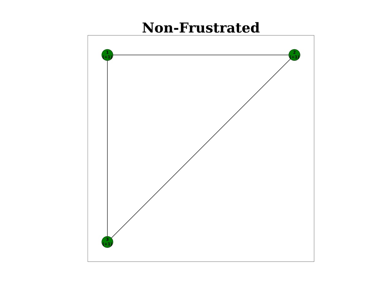
| Configuration $S_{i}$ | $H(S_{i}, J)$ | $\mathbb{P}(S_{i})$ | |
|---|---|---|---|
| A | $\left[1,1,1 \right]$ | $-3$ | $\frac{e^{3\beta}}{2e^{3\beta} + 6e^{-\beta}}$ |
| B | $\left[1,1,-1 \right]$ | $+1$ | $\frac{e^{-\beta}}{2e^{3\beta} + 6e^{-\beta}}$ |
| C | $\left[1,-1,1 \right]$ | $+1$ | $\frac{e^{-\beta}}{2e^{3\beta} + 6e^{-\beta}}$ |
| D | $\left[1,-1,-1 \right]$ | $+1$ | $\frac{e^{-\beta}}{2e^{3\beta} + 6e^{-\beta}}$ |
| E | $\left[-1,1,1 \right]$ | $+1$ | $\frac{e^{-\beta}}{2e^{3\beta} + 6e^{-\beta}}$ |
| F | $\left[-1,1,-1 \right]$ | $+1$ | $\frac{e^{-\beta}}{2e^{3\beta} + 6e^{-\beta}}$ |
| G | $\left[-1,-1,1 \right]$ | $+1$ | $\frac{e^{-\beta}}{2e^{3\beta} + 6e^{-\beta}}$ |
| H | $\left[-1,-1,-1 \right]$ | $-3$ | $\frac{e^{3\beta}}{2e^{3\beta} + 6e^{-\beta}}$ |
Here we can satisfy all constraints, and we have two ground states with $H = - 3$: all spins up or down. On the other hand, adding a negative coupling to this system gives a frustrated system:
\[J = \begin{bmatrix} 0 & -1 & 1 \\ -1 & 0 & 1 \\ 1 & 1 & 0 \end{bmatrix}\]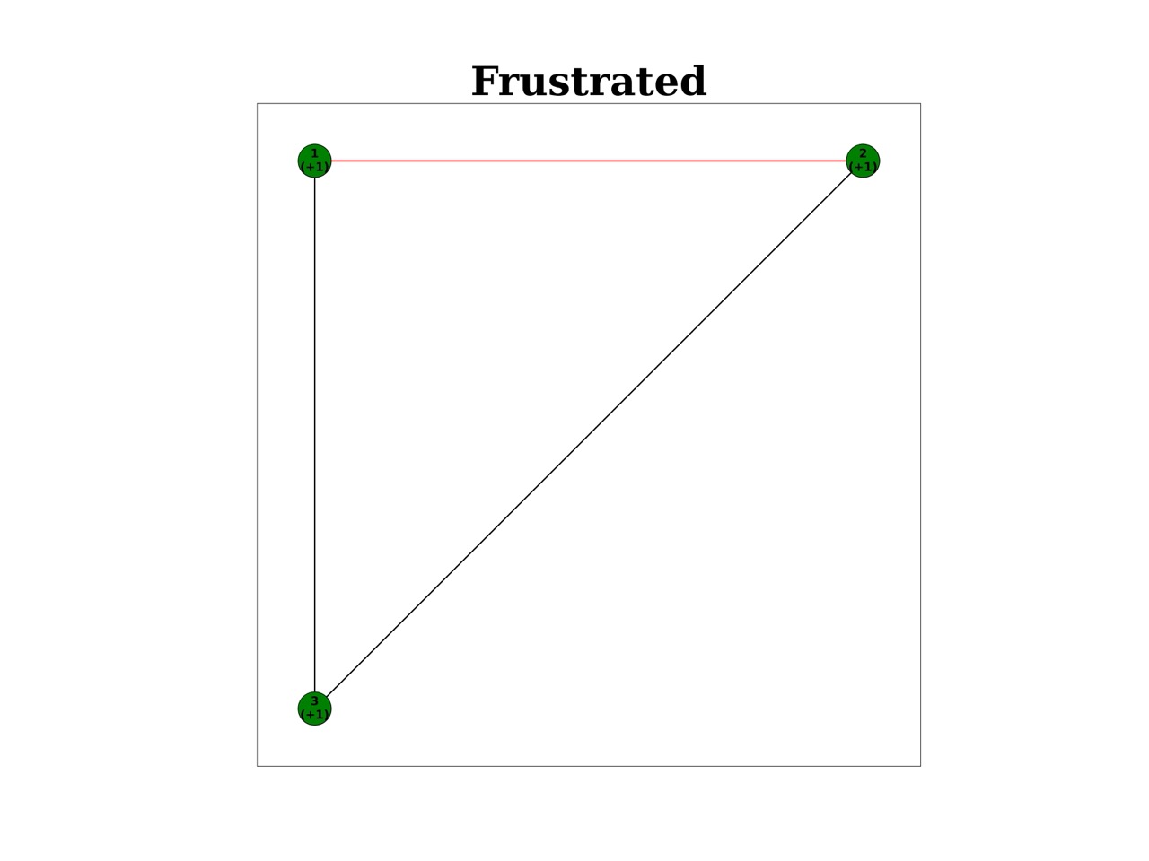
We can compute the Hamiltonian and Boltzmann probability for each state
| Configuration $S_{i}$ | $H(S_{i}, J)$ | $\mathbb{P}(S_{i})$ | |
|---|---|---|---|
| A | $\left[1,1,1 \right]$ | $-1$ | $\frac{e^{\beta}}{6e^{\beta} + 2e^{-3\beta}}$ |
| B | $\left[1,1,-1 \right]$ | $+3$ | $\frac{e^{-3\beta}}{6e^{\beta} + 2e^{-3\beta}}$ |
| C | $\left[1,-1,1 \right]$ | $-1$ | $\frac{e^{\beta}}{6e^{\beta} + 2e^{-3\beta}}$ |
| D | $\left[1,-1,-1 \right]$ | $-1$ | $\frac{e^{\beta}}{6e^{\beta} + 2e^{-3\beta}}$ |
| E | $\left[-1,1,1 \right]$ | $-1$ | $\frac{e^{\beta}}{6e^{\beta} + 2e^{-3\beta}}$ |
| F | $\left[-1,1,-1 \right]$ | $-1$ | $\frac{e^{\beta}}{6e^{\beta} + 2e^{-3\beta}}$ |
| G | $\left[-1,-1,1 \right]$ | $+3$ | $\frac{e^{-3\beta}}{6e^{\beta} + 2e^{-3\beta}}$ |
| H | $\left[-1,-1,-1 \right]$ | $-1$ | $\frac{e^{\beta}}{6e^{\beta} + 2e^{-3\beta}}$ |
We see there are 6 degenerate ground states at higher energy, $H = -1$.
Random frustrated Lattice
Increasing the size of our system to $N=16$ but considering only local interactions on a lattice, we are still able to brute-force compute the energy landscape across configuration space.
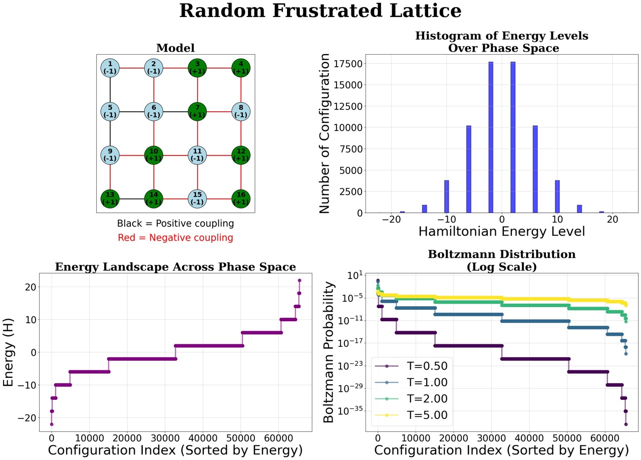
Here we see we have a few low energy configurations, many moderate energy configuration, and a few high energy configurations. However, notice the average energy across configuration space is $H=0$. Based on the Boltzmann probabilities, it’s clear the system is much more likely to be in some configurations (the low energy ones).
Sherrington-Kirkpatrick Model
Now we introduce a model that more closely models a physical spin glass, the Sherrington-Kirckpatrick (SK) spin glass model. To simplify things, the SK uses what is called a mean field approximation. This means every node interacts with some mean field of the rest of the system, rather than having distinct local and sparse interactions. We continue to deal with Ising spins, where we assume the spin state of each variable $i$ is $\sigma_{i} = \pm1$.
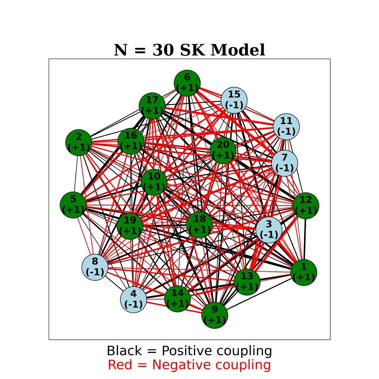
To construct the coupling matrix $J$, we draw each $J_{ij}$ from a zero mean, i.i.d Gaussian distribution with variance $1/N$. For example, the coupling matrix of a SK model with 4 degrees of freedom may look like:
\[J = \begin{bmatrix} 0 & 0.015 & -0.687 & 0.0139 \\ 0.0159 & 0 & 0.091 & -0.017 \\ -0.687 & 0.091 & 0 & 0.058 \\ 0.019 & 0.016 & -0.158 & 0 \end{bmatrix}\]The coupling between ions $i$ and $j$, $J_{ij}$ indicates the desired relationship between their spins:
\[J_{ij} > 0: \text{the spins should be of the same sign}\] \[J_{ij} < 0: \text{the spins should be of the opposite sign}\] \[|{J_{ij}}| \text{ determines the strength of the relationship}\]We can again compute the Hamilton and Boltzmann distribution across configuration space:
We find a similar pattern to the frustrated lattice. Next we introduce a few more measures that can tell use about the phase state of the system. In other words, the level of order in the system.
Order Parameters
Definition (Magnetization):
An order parameter that measures the average spin per site. This is an indication of “up-ness” or “down-ness” of the system. If the magnetization is $1$ or $-1$, the system is in a paramagnetic phase.
\[M = \frac{1}{N}\sum_{i} \left\langle \sigma_i \right\rangle\]In the SK model, $M \simeq 0$ at equilibrium, since $J_{ij}$ are drawn from a zero-mean Gaussian. This makes magnetization a poor order parameter for distinguishing the spin glass phase from the paramagnetic phase, and motivates introducing the Edwards-Anderson order parameter.
Definition (Edwards-Anderson Order Parameter):
\[q_{EA} = \frac{1}{N}\sum_{i}^{N} \left\langle \sigma_i \right\rangle ^2\]This captures whether individual spins have frozen into a definite direction on average, even if those directions are random across sites. This will distinguish the spin-glass phase.
For example, in the SK model if we compute the
The Free Energy
Definition (Free Energy):
With the partition function, we can define a energy measure of the entire system that is independent of an individual configuration, called the free energy.
\[F(J) = -T \text{ ln } Z(J)\]The free energy encodes all equilibrium thermodynamic properties of the system, and you can derive magnetization and $q_{EA}$ from it by taking the appropriate derivatives. So computing $F$ is essentially solving the system. We will see the free energy is central to the replica method. Note however that computing the free energy requires finding the partition function. Some toys systems are exactly solvable, but in general the configuration space is too large for this to be feasible.
Ways to Analyze a Statistical Mechanical System:
| Approach | Pros | Cons |
|---|---|---|
| 1. Brute Force | Exact, tells us about all possible configurations | Computationally intractable, does not tell us about equilibrium. |
| 2. Monte Carlo Sampling | Efficient and simple, represents behavior at thermodynamic equilibrium | Only tells us about a single walk, may get stuck in local energy minima. |
| 3. Replica Method | Exact, analytic solution that tells us about all equilibrium configurations | Difficult to solve, requires an ansatz (assumption) about the overlap of equilibrium configurations to solve. |
So far we have looked at some measures over the configuration space of the system. However, in reality the system will tend towards the small number of low energy configurations at thermodynamic equilibrium. Additionally, computing the partition function becomes increasingly computationally expensive as $N$ gets large. One solution is to use Monte Carlo simulation, as we explore next.
Monte Carlo Simulation of Statistical Mechanical Models
We can approximate a models’ Boltzmann distribution without computing the partition function directly. We will use Monte Carlo simulation and the Metropolis-Hastings Algorithm to sample the Boltzmann distribution. This chain of samples will form a single walk through the configuration space that tends towards the equilibrium low energy configuration.
Metropolis-Hastings Algorithm
-
Initialize the model in a random configuration
-
Propose flipping one spin and calculate $\Delta H = H_{new} - H_{old}$
-
Choose to accept or reject the move:
- $ \Delta H \le 0$: always accept it
- $ \Delta H > 0$: accept with $P(accept) = e^{(\beta \Delta H)}$
-
Take many of these steps
The dynamical progression of the system through configuration space here will follow the Boltzmann probability of the system instantiating a particular configuration. Over time, the system will try to minimize energy, and approach an equilibrium average energy, $H_{eq}$. This process depends on the temperature of the system: if temperature is high, $\beta$ is small, and therefore the effect of positive $\Delta H$ (increasing the energy of the system) on the probability of accepting that state is higher. With high thermal energy, the system will explore more of the configuration space, and have a higher $H_{eq}$. I implemented this algorithm in python and simulated the evolution of the lattice and SK systems.
Simulating the Lattice:
Here we see that a non-frustrated lattice will tend towards lower energy configurations from a random initialization. This is however temperature dependent: at $T=5.0$, the system has enough thermal energy to continuously explore the configuration space, and its $H_{eq}$ is around where it was initialized, $H \sim -300$. On the other hand, the lower temperature systems tend towards lower energy configurations. As expect, the opposite effect is seen on absolute average magnetization per spin. At low energy, the system equilibrates into the low energy paramagnetic phase. Interestingly, note that these results are not perfect: at $T=1.0$, the system enters a low energy well below $T=2.0$ and seems to get stuck there, though absolute magnetization remains lower than in $T=2.0$. This illustrates an important point: Monte Carlo Sampling only tells us about a single random walk through the space. If the system is initialized in a local energy minima, at low temperatures it may remain stuck there.
In the frustrated lattice, we see $H_{eq}$ still settles down to temperate dependent values, though overall average energy is increased. In the magnetization plot, we see the characteristic chaotic behavior of a frustrated system. Magnetization remains low at all temperatures, and fluctuates quite randomly. The system is stuck in a spin glass phase and cannot transition into a stable paramagnetic phase.
Simulating the SK Model
The results for the SK model resemble those of the frustrated lattice, though magnetization appears slightly more chaotic, especially at low temperatures. This make sense given the greater degree of frustration from the dense, randomly drawn couplings.
The main takeaway is that though Monte Carlo simulation can give us a sense for the $H_{eq}$ of a spin glass system, it cannot tell us about the global, configuration space wide behavior of such system. In other words, each simulation is limited to a specific instantiation of the system, and the trajectory of a single system through configuration space. It cannot tell us much about the pockets of low energy minima that are scattered across the jagged energy landscape associated with that space, nor the average behavior across all possible configurations. Enter replica theory!
The Replica Method
The replica method is an analytic approach to understanding the equilibrium properties of the SK model. It is chiefly concerned with understanding the free energy landscape of the system averaged over all possible couplings $J$. The free energy is self averaging, meaning that if we compute its average over the set of all possible couplings, we understand it for a typical realization of $J$.
We are interested therefore in determining the quenched average over disorder:
\[\left\langle \left\langle F(J)\right\rangle \right\rangle_{\mathscr{J}} = \left\langle \left\langle -T \text{ ln } Z(J)\right\rangle \right\rangle_{\mathscr{J}}\]This is hard becasue the log is inside the average. We exploit the identity
\[\text{ln } Z = \lim_{n \to 0} \frac{Z^{n} -1}{n} = \lim_{n\to 0} \frac{\partial}{\partial n} Z^{n}\]where we treat $( Z^{n})$ as the partition function for n replicas of the same sample. Then it is possible to average over an integer power of $Z(J, \beta)$ and take the $n \rightarrow 0$ limit. This is the most controversial step of the Replica method, and is not strictly the most rigorous maneuver. We introduced $Z^n$ as the partition function for $n\in \mathbb{N}$, $n > 0$ replicas, and then take an analytic continuation to zero. However, Replica Theory makes remarkably accurate empirical predictions despite this concern.
Now remember that
\[Z(J, \beta) = \sum_{S}e^{-\beta H(S,J)} =\sum_{S}e^{\beta \sum_{i \lt j} J_{ij}\sigma_{i}\sigma_{j}}\]We introduce $n$ identical but distinct configurations $S^a$ for $a =1,\dots,n$ and multiply their partition functions:
\[Z^{n} = \left( \sum_{\left\{S^{1}\right\}} e^{\beta \sum_{i<j}J_{ij}\sigma_{i}^{1}\sigma_{j}^{1}} \right) \times \left( \sum_{\left\{S^{2}\right\}} e^{\beta \sum_{i<j}J_{ij}\sigma_{i}^{2}\sigma_{j}^{2}} \right) \times \cdots \times \left( \sum_{\left\{S^{n}\right\}} e^{\beta \sum_{i<j}J_{ij}\sigma_{i}^{n}\sigma\_{j}^{n}} \right)\]We then take the average over $\mathscr{J}$:
\[\left\langle \left\langle Z^{n} \right\rangle \right\rangle_{\mathscr{J}} =\left\langle\left\langle \sum_{\left\{ S^{1},...,S^{n} \right\}}e^{\beta \sum_{a=1}^{n}\sum_{i \lt j} J_{ij}\sigma_{i}^{a}\sigma_{j}^{a}} \right\rangle \right\rangle_{\mathscr{J}}\]Due to the fact that the couplings were drawn from a Gaussian distribution, this average can be performed because it can be reduced to Gaussian integrals with the identity
\[\left\langle e^{zx} \right\rangle_z = e^{1/2\sigma^2x^2}\]Where $z$ is a zero mean Gaussian with variance $\sigma^2$.
Results From the Replica Method
Many deep results emerge from Replica Theory that are beyond the scope of this article. I refer the reader to the references for in depth explanation. Briefly, the solution to this problem depends on the structure of the overlap matrix $Q_{ab}$ which describes overlap between two replicas $a$ and $b$. The replicated partition function can be rewritten as a function of $Q_{ab}$, yeilding
\[\left\langle \left\langle Z^{n} \right\rangle \right\rangle_{\mathscr{J}} = \int \prod_{(ab)} \frac{dQ_{ab}}{2\pi}e^{N\mathcal{A}[Q_{ab}]}\]At the thermodynamic limit ($N \rightarrow \infty$), this integral can be evluated via the Laplace or saddle-point methods. Since the results depend on $Q_{ab}$, one must assume an ansatz for its strucutre. This reveals a number of magnetic regimes that describe the free energy landscape of this system as it undergoes phase transitions.
Replica Symmetric (RS)
In this case overlap among different replicas is the same for any pair of replicas, except between a replica and itself. $Q_{ab}$ admits only two values: diagonal contribution $q_{d} \text{ for } a = b$ and off diagonal $q_{0} \text{ for } a \not = b$
This correctly describes high temp, large external field regimes. However, as these parameters are lowered, some models reach critical a critical de Almeida-Thouless (dAT) line, below which RS solutions become unstable, and a spin glass phase emerges.
Replica Symmetry Breaking (RSB)
Below the dAT line, correct solution requires a matrix $Q_{ab}$ with an iterative block structure, which breaks the symmetry between different pairs of replicas. This procedure can reveal the organization of the free energy landscape. For example, the Parisi solution to the SK model at low temperatures reveals a complex, hierarchical, and ultrameric structure to the phase space. Parisi’s method of breaking the symmetry multiple times (k-step RSB), up to an infinite number of times (full-RSB) correctly describes the system at any temperature.
Conclusion
Here I hope to have motivated the power of the Replica Method in analyzing complex systems with many interacting degrees of freedom. Though Monte-Carlo simulations can tell us about the average behavior of the system, this method is quite limited. Replica theory develops a picture that reveals a deep structure in the energetics of a chaotic spin glass system like the SK model, which intuitvely seems like it would be random without significant organization. The implications of this theory extend deeply into problems in machine learning, neuroscience, and optimization, and represent a promising direction of ongoing research.
References
Advani, M., Lahiri, S., Ganguli, S., 2013. Statistical mechanics of complex neural systems and high dimensional data. J. Stat. Mech. 2013, P03014. https://doi.org/10.1088/1742-5468/2013/03/P03014
Altieri, A., Baity-Jesi, M., 2023. An Introduction to the Theory of Spin Glasses.
Daniel Schroeder, 2000. An Introduction To Thermal Physics.
Engel, A., 2004. Statistical Mechanics of Learning.
The Ising Model [WWW Document], n.d. URL https://stanford.edu/~jeffjar/statmech/intro4.html (accessed 6.30.25).