Project background

This document encapsulates my work in the University of Illinois Chicago department of Mathematics, Statistics, and Computer Science’s Spring 2025 Directed Reading Program (DRP). I presented a version of this material in a short talk at the conclusion of the semester. I was mentored by Jennifer Vaccaro, and am deeply grateful for her continued support and mentorship in this program! This DRP was co-organized by Yijia Chen, Nick Christo, Clay Mizgerd, and Michael Gintz.

Slides from my presentation

DRP website

Abstract

Graph Convolutional Networks (GCNs) are a scalable and efficient machine learning approach to semi-supervised learning on graph structured data. GCNs are used to classify graphs based on their features by aggregating information across adjacent nodes according to learnable parameters. They are a powerful tool which extends the concept of convolution on grid structured data (i.e. image processing contexts) to graph structured data. This finds applications in tasks including functional brain connectivity analysis, node classification, molecular property prediction, and link prediction.

Introduced by Thomas Kipf and Max Welling in their 2016 paper Semi-Supervised Classification with Graph Convolutional Networks, the architecture emerges from a localized first-order approximation of spectral graph convolutions. This model learns hidden layer representations that encode information about local graph structutre and node features, enabling the model to learn complex features of the graph, and in turn the various abilities of GCNs.

Primary Texts

Graph Representation Learning - William L. Hamilton (2020)

Semi-Supervised Classification with Graph Convolutional Networks - Kipf & Welling (2016)

CNNs and Image Convolution

I will start with a slightly simpler type of model: the Convolutional Neural Network (CNN). Traditional CNNs operate over grid structured data such as image pixel matrices, and learn hidden layer representations that encode features of the input grid and enable the model’s application in various tasks. These types of model have found widespread use in computer vision, though they have uses in any setting where the data can be structured as a euclidean grid.

Convolution of images

Every image is a grid of nicely aranged pixels which each have some value $x_{i}$ associated with them. In the case of greyscale images, this is a single value between 0 and 1. In color images, $x_{i} = <r,g,b>$ is a vector encoding the red, green, and blue values.

The main component of convolution is the kernel, which is simply another (typically smaller) grid with a defined weight for each entry. In one convolutional step, the kernel is passed over the entire image as partially illustrated below.

Grid convolution

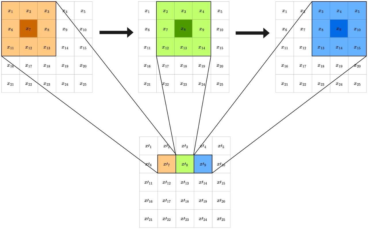
At each step as the kernel moves, a new value $x’{i}$ is generated for each pixel by _convolving the filter weights with the pixel values, which just means taking a weighted linear combination of each pixel’s immediate neighbors. Once the kernel has been passed across the entire image, the effect is that information is spread across pixels, based on the chosen weights.

kernel on grid

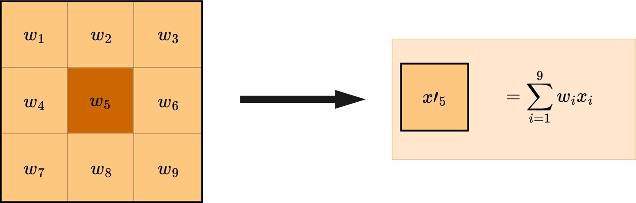
The kernel weights determine what information is picked out by the convolution

Different weights lead to different effects on the image. The simplest filter simply blurs the image (averages information across pixels), while other weights pick out features such asverticle edges, horizontal edges, etc.

image convolution

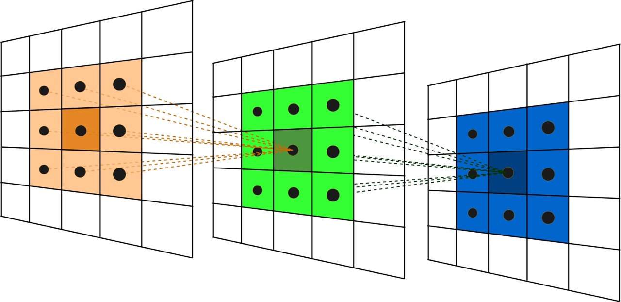
Convolutional Neural Networks

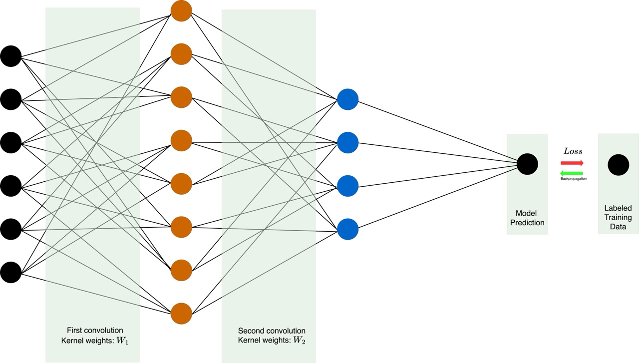
When constructing a CNN, multiple convolutional steps are combined, and unique kernel weights are learnt at each hidden layer. As a result the network is able to complex, hierarchial feautures of the image. The interlayer connectivity of neurons in the network is impacted by the size of the kernel (2x2, 3x3, etc.), but is fundamentally determined by the local proximity of pixels. The weights of these connections are the parameters learnt by the model in training.

3dCNN

In training, the output of the model is compared to the human-labelled classification for a number of examples via a loss function $\mathcal{L}$. When the model is wrong, $\mathcal{L}$ is large, when the model is correct, $\mathcal{L}$ is small.

In the simplest situation of image recognition, the classification is a single value representing the probability the image is a given thing, but in reality could be a vector in $\mathbb{R}^{C}$. For example, in hand written digit recogition, the output $\vec{O} \in \mathbb{R}^{9}$ encodes the probability a given digit is $0,…,9$.

Various types of loss functions exist and may be prefered depending on the specific application and details of the classification (binary vs. categorical). A loss function commonly used in classification is Cross Entropy Loss.

For N instances (training examples):

Binary Cross Entropy: $ \mathcal{L} = -\frac{1}{N} \sum_{i=1}^{N}(l_{i} log(o_{i}) +(1-l_{i})log(1-o_{i})) $

Where

$l_{i}$ - true label for instance $i$
$o_{i}$ - predicted probabilty by model for instance $i$

Multiclass Cross Entropy: $ \mathcal{L} = -\frac{1}{N} \sum_{i=1}^{N}\sum_{j=1}^{C}(l_{i,j} log(o_{i,j}) $

Where

C is the number of classes
$l_{i,j}$ - true labels for class $j$ for instance $i$
$o_{i,j}$ - predicted probabilty by model for class $j$, for instance $i$

Using this loss function, the weights of the model are updated with the backpropogation algorithm, such that $\mathcal{L}$ is minimized. Over a large number of training examples, the model learns the optimal parameters within the given arcihitecture to correctly classify input images.

Abstractly, at each layer, the model learns to extract some useful feature in order to classify the image.

cnn

Graph Convolutional Networks

We can extend the same idea from grids to irregular graphs, however it is more complicated. We can think of grids as special, highly-regular graphs, where each pixel is a node connected to all of its immediate neighbors:

gcn

In grid convolution, the kernel defines both the neighboorhood over which information is aggregated (in this case the 1-hop neighborhood), and the weight of each neighbor’s contribution to the update. In graph convolution, we will do this in two steps instead of one. First, we will define the message passsing algorithim, which gives us a way of spreading information across the structural neighborhoods of the graph, and then we use a seperate weight matrix that allows the model to learn to extract meaningful features.

Message passing on graphs:

The message passing algorithm provides a way to distribute feature information between nodes of a graph based on the structure of the graph. Each node in the graph has a feature vector $\vec{x_{i}}$, which it sends out to its neighbors, and each node recieves a signal from its neighbors. After message passing, the updated feature vector $\vec{x’_{i}}$ is some combination of its own message and its neighbors’.

message_passing

This can be done mathematically by multiplying the adjacency matrix of the graph (with self loops) $\tilde{A}$ by a matrix $H^{(l)}$ whose $i-th$ row is the feature vector of the $i-th$ node in layer $l$.

\[\begin{aligned} &H^{(l+1)} = \widetilde{A}H^{(l)} = \begin{bmatrix} 1 & 1 & 1 & 1 \\ 1 & 1 & 0 & 0 \\ 1 & 0 & 1 & 0 \\ 1 & 0 & 0 & 1 \end{bmatrix} \begin{bmatrix} \vec{x}_1 \\ \vec{x}_2 \\ \vec{x}_3 \\ \vec{x}_4 \end{bmatrix} = \left[ \begin{array}{l} \vec{x}_1 + \vec{x}_2 + \vec{x}_3 + \vec{x}_4 \\[6pt] \vec{x}_1 + \vec{x}_2 \\[6pt] \vec{x}_1 + \vec{x}_3 \\[6pt] \vec{x}_1 + \vec{x}_4 \end{array} \right] \\ &\scriptsize{(\text{Where } \widetilde{A} = A + I)} \end{aligned}\]

The result of this is exactly what we wanted - each node’s features are a combination of their own and their neighbors feautures in the last layer. However, this simply sums up feature information, and as such these values will grow larger and larger as further convolutions are performed. Additionally, due to the irregularity of the graph, some nodes have more neighbors and will accumlate information more quickly. This poses problems to training, namely exploding/vanishing activations and gradients.

Degree Normalization

To account for this, $\tilde{A}$ is normalized by the degree of each node, that is, how many neighbors each node has. The normalized adjacency is: $\hat{A} = \tilde{D}^{-\frac{1}{2}}\tilde{A}\tilde{D}^{-\frac{1}{2}}$, where $\tilde{D}$ is a diagonal matrix that encodes the degree information of the graph with self-loops.

\[\widetilde{D} = \begin{bmatrix} 4 & 0 & 0 & 0 \\ 0 & 2 & 0 & 0 \\ 0 & 0 & 2 & 0 \\ 0 & 0 & 0 & 2 \end{bmatrix} \quad \longrightarrow \quad \widetilde{D}^{-\frac{1}{2}} = \begin{bmatrix} \frac{1}{2} & 0 & 0 & 0 \\ 0 & \frac{1}{\sqrt{2}} & 0 & 0 \\ 0 & 0 & \frac{1}{\sqrt{2}} & 0 \\ 0 & 0 & 0 & \frac{1}{\sqrt{2}} \end{bmatrix} \quad \longrightarrow \quad \widetilde{D}^{-\frac{1}{2}} \widetilde{A} \widetilde{D}^{-\frac{1}{2}} = \begin{bmatrix} \frac{1}{4} & \frac{1}{\sqrt{8}} & \frac{1}{\sqrt{8}} & \frac{1}{\sqrt{8}} \\[6pt] \frac{1}{\sqrt{8}} & \frac{1}{2} & 0 & 0 \\[6pt] \frac{1}{\sqrt{8}} & 0 & \frac{1}{2} & 0 \\[6pt] \frac{1}{\sqrt{8}} & 0 & 0 & \frac{1}{2} \end{bmatrix}\]

In spectral terms, this has the effect of ensuring the eigenvalues of $\hat{A}$ are between 0 and 1, which avoids the aforementined issues when training the model. This is made clear when we simply do the same message passing step as before, but with the degree normalized adjacency this time:

\[H^{(l+1)} = \underbrace{ \widetilde{D}^{-\frac{1}{2}} \widetilde{A} \widetilde{D}^{-\frac{1}{2}} }_{ \text{Entry } (i,j) = \frac{\widetilde{a}_{ij}}{\sqrt{d_i d_j}} } H^{(l)} = \left[ \begin{array}{l} \frac{1}{4}\vec{x}_1 + \frac{1}{\sqrt{8}}\vec{x}_2 + \frac{1}{\sqrt{8}}\vec{x}_3 + \frac{1}{\sqrt{8}}\vec{x}_4 \\[6pt] \frac{1}{\sqrt{8}}\vec{x}_1 + \frac{1}{2}\vec{x}_2 \\[6pt] \frac{1}{\sqrt{8}}\vec{x}_1 + \frac{1}{2}\vec{x}_3 \\[6pt] \frac{1}{\sqrt{8}}\vec{x}_1 + \frac{1}{2}\vec{x}_4 \end{array} \right]\]

This enables the model to project the features into various linear feature spaces at different layers and extract meaningful patterns/structural features. Over the course of learning, these weight matrices are tuned to minmize the loss.

The only remaining thing to get to a complete GCN layer is to wrap this entire expression in a non-linear function, such as the sigmoid ($\sigma$) or rectified linear unit (ReLU) function.

\[H^{(l+1)} = \underbrace{\sigma}_{\substack{\text{Non-linear Activation} \\ \text{Function}}} \left( \widetilde{D}^{-\frac{1}{2}} \widetilde{A} \widetilde{D}^{-\frac{1}{2}} H^{(l)} W^{(l)} \right)\]

This activation function acts element wise on the output of the matrix multiplications, acting to either threshold the activations above zero (ReLU), or to restrain them to between 0 and 1 ($\sigma$), as shown below. These functions are essential in enabling the model to exhibit non-linear behavior and learn to classify highly complex graphs, despite being made up primarily of linear operations.

activation

Conclusion:

The conceptual framework of Convolutional Neural Networks used in image recognition can be used to understand the function of Graph Convolutional Networks and their operation on irregular graph data. The adjacency matrix encodes the structure of the graph, and provides a way to spread feature information across nodes based on their connectivity. Degree normalization controls for differential connectivity of various nodes, and linear projection matrices are the parameters which allow the model to learn. These matrices are tuned during training, and allow the model to extract and make use of highly complex features of graph structure and feature information in learning how to classify graphs, or perform other tasks.

References

Daigavane, Ameya, Balaraman Ravindran, and Gaurav Aggarwal. 2021. “Understanding Convolutions on Graphs.” Distill 6 (9): e32. https://doi.org/10.23915/distill.00032.

Hamilton, William L. 2020. “Graph Representation Learning.”

Jiang, Hao, Peng Cao, MingYi Xu, Jinzhu Yang, and Osmar Zaiane. 2020. “Hi-GCN: A Hierarchical Graph Convolution Network for Graph Embedding Learning of Brain Network and Brain Disorders Prediction.” Computers in Biology and Medicine 127 (December):104096. https://doi.org/10.1016/j.compbiomed.2020.104096.

Kipf, Thomas N., and Max Welling. 2017. “Semi-Supervised Classification with Graph Convolutional Networks.” arXiv . https://doi.org/10.48550/arXiv.1609.02907.

Sanchez-Lengeling, Benjamin, Emily Reif, Adam Pearce, and Alexander B. Wiltschko. 2021. “A Gentle Introduction to Graph Neural Networks.” Distill 6 (9): e33. https://doi.org/10.23915/distill.00033.

Wilson, Robin J. 1972. Introduction to Graph Theory. New York, Academic Press. http://archive.org/details/introductiontogr00wils.